In the past week or so, we’ve set up the baseline parallel interface and implementation, compatible with OCaml’s stdlib. We have a drop-in replacement for OCaml’s stdlib’s map and set operations, with parallelism enabled. We implemented this baseline parallel version using OCaml domains, as anticipated in our proposal, which we can tweak as needed (i.e., change the number of parallel workers). Our focus up to this point has been understanding the problem in more depth (and understanding OCaml) to be able to flag any issues during the remaining half of the project so that we could pivot if needed (so far this has not been the case, thankfully). Additionally, our goal has been making sure our benchmarking and testing setup is as sound as possible so we don’t waste time in the final weeks tweaking our setup. We decided on a single consistent set of benchmarks and tests so we can track the impact of optimizations better (this is particularly important for our project since a major component will be understanding how OCaml’s generational garbage collector interacts with the parallelism we introduce; using the same subset of major benchmarks will help us better isolate behavior).
To this end, we’ve set up a set of five benchmark workloads (e.g., random equal-sized sets of data, disjoint data, clustered data, etc.) which we’ll describe in more depth in our final report. We call these input configurations (ICs). Running the parallel implementation on these benchmarks (and comparing correctness directly with the stdlib implementation), we have some preliminary speedup graphs and GC performance data (see below; ran on a local M1 MacBook Pro). As predicted in our proposal, the GC begins to limit parallelism significantly at higher thread/worker counts, which we’ll start investigating in more depth over the next couple of weeks. At the moment, the parallel implementation is a naive port of the stdlib approach with a configurable granularity cutoff. The current speedup graphs are run without a tuned granularity cutoff (currently just set to 1, which is the height of the smallest balanced tree used for the internal representation of the set/map; more details on this in our report). We have also attached some plots on some sweeps we’ve started running to find a more optimal granularity cutoff.
While we are on schedule with our implementation and preliminary data (see our schedule below for some of the areas we are hoping to explore and add), we do have a couple of concerns as we head into the final half of the project. Namely, the depth of optimization we can achieve given OCaml’s high-level language constructs. This is an inherent concern we’ve kept in mind since the beginning, so it’s not a huge surprise, but we just need to figure out how much of our analyses can actually result in meaningful optimization targets under OCaml’s more restrictive programming model (as opposed to in-class uses of C/C++). We are optimistic based on the implementation so far (though we haven’t gotten to any in-depth optimizations yet). It is entirely possible that many optimizations will be moot given the inherent costs of synchronization in the OCaml GC and the amount of work being done by the more complex compiler. Additionally, since we are trying to maintain a fair comparison with the stdlib implementation, restricting our data structures slightly, we hope there isn’t so much restriction that we hit a wall too early. Nonetheless, we are optimistic as we’ve already gained some new insights on parallelizing in a very different runtime system.
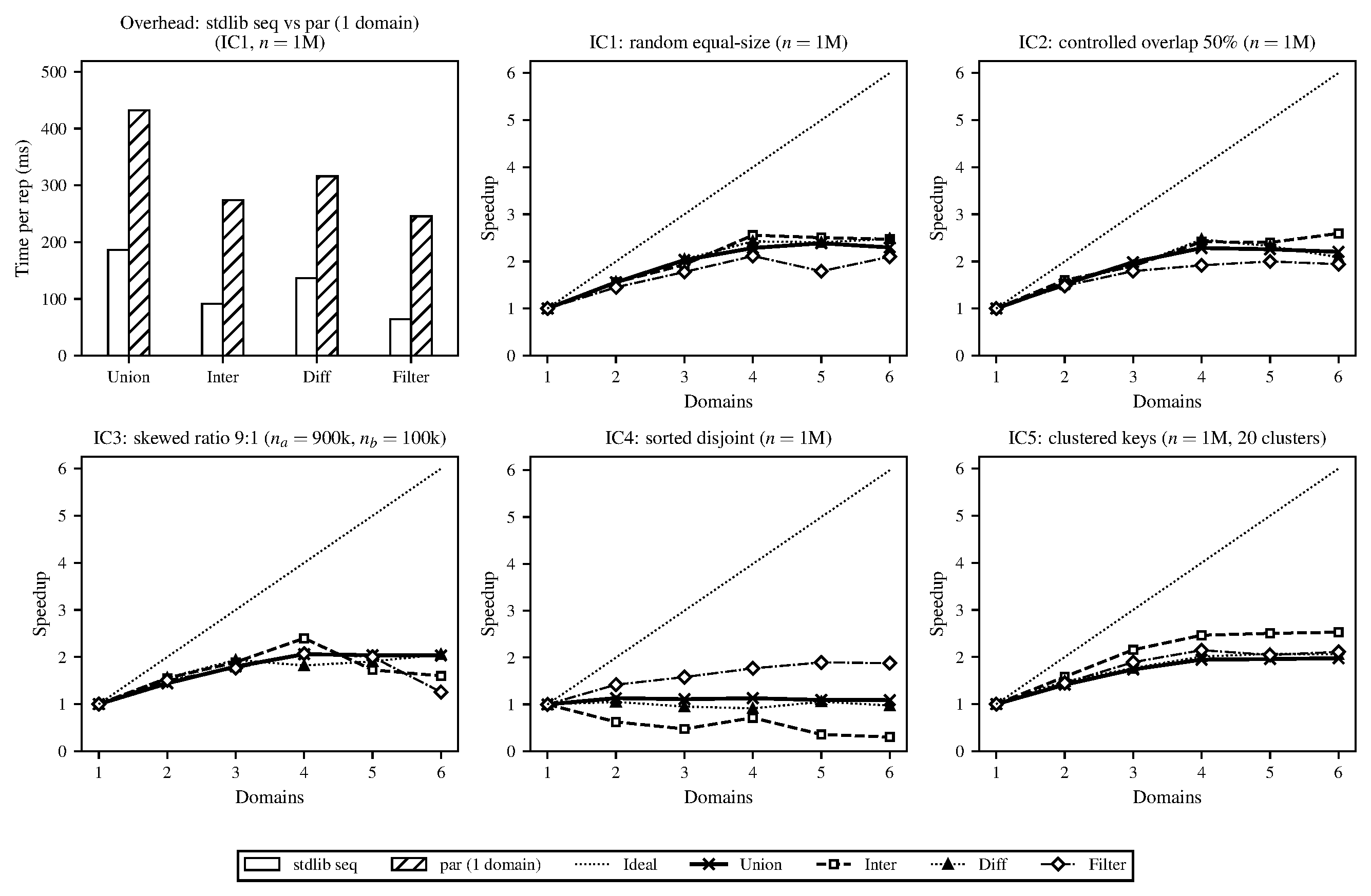
Figure 1. Speedups of domain-based implementation, averaged over 10 repetitions, smallest granularity (cutoff height).
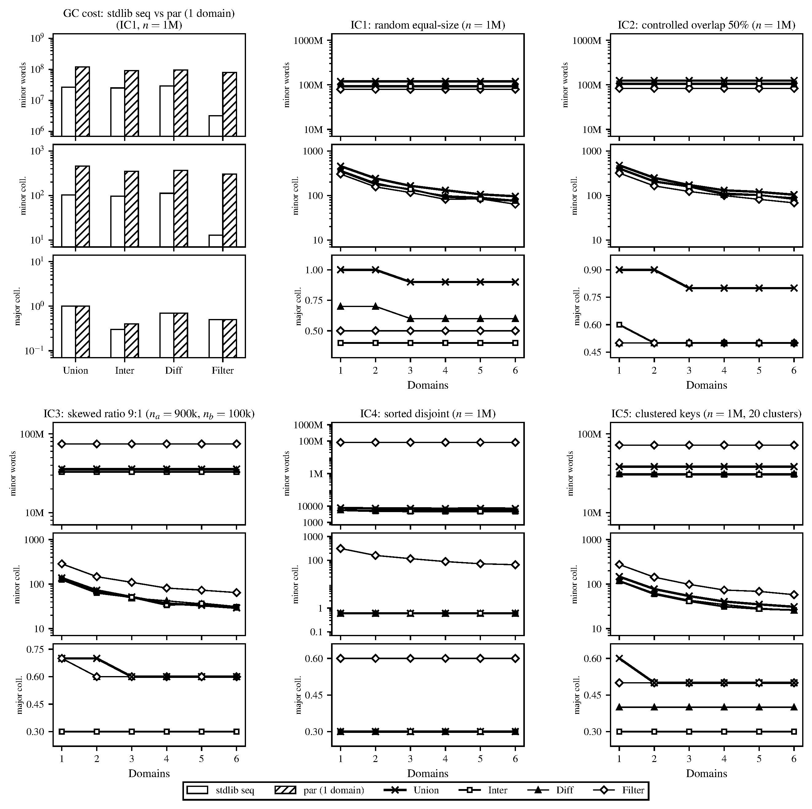
Figure 2. GC statistics of domain-based implementation, averaged over 10 repetitions, smallest granularity (cutoff height).
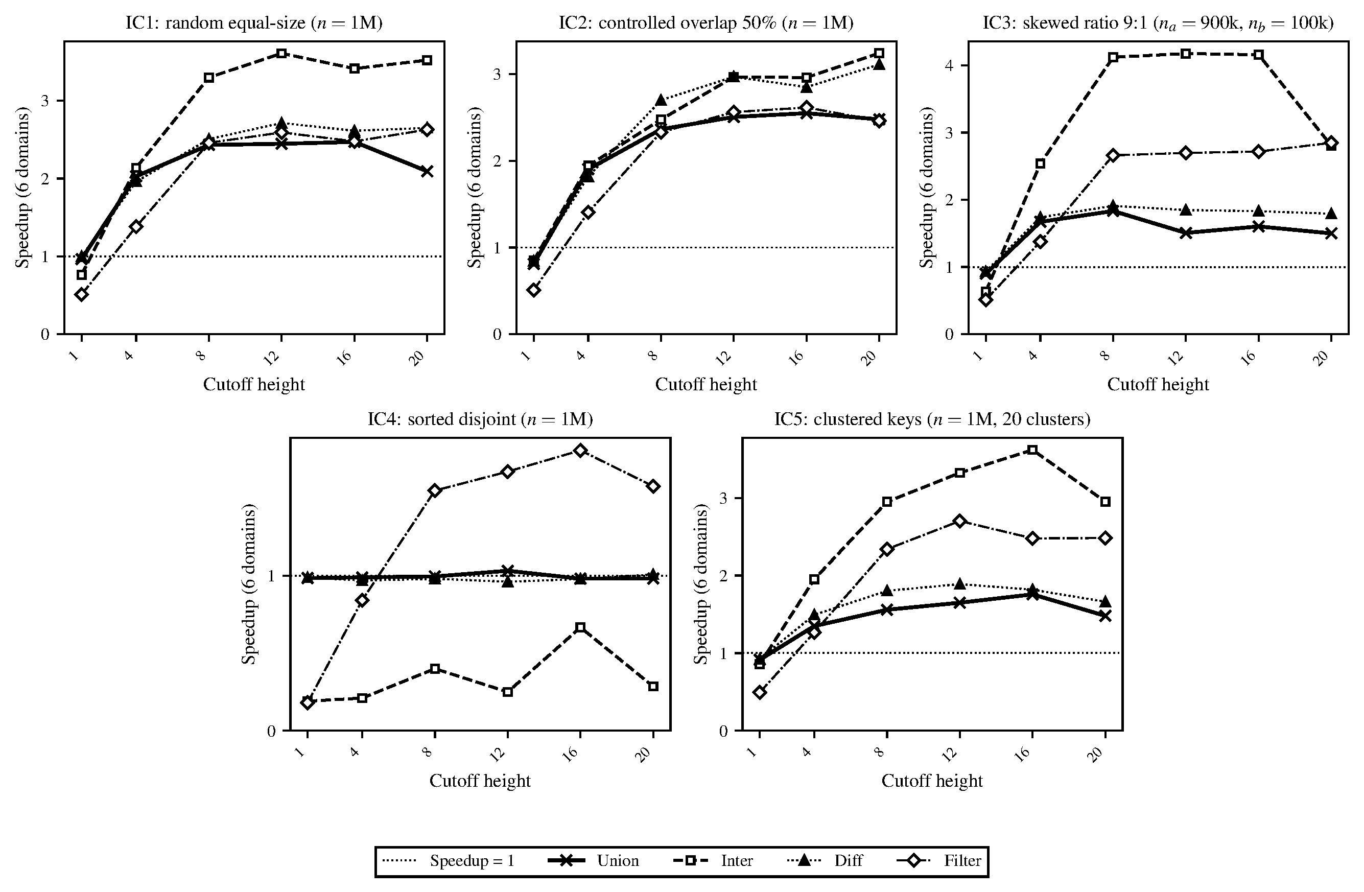
Figure 3. Sweep to find speedup-optimal task granularity (tree height cutoff), averaged over 8 repetitions.
(The outline below is subject to change, as we are not yet sure of all the optimizations we will use.)
- 4/15 – 4/18: Begin optimizing and profiling. The goal is to profile the current parallel implementation to identify the main bottlenecks, test whether tuning the OCaml garbage collector helps, and test out some smaller algorithmic shortcuts.
- Simon’s focus: Sweep OCaml’s minor heap size to check whether larger heaps reduce GC pressure on our workload. Implement an early-exit in parallel intersection and difference that skips some recursion. Try to measure what fraction of the
unionoperation is spent in each phase of the recursion. - Michael’s focus: Figure out whether OCaml 5 and its parallelism library can be installed on the GHC machines (or PSC), then collect some HW perf counter data to figure out whether the parallel implementation is limited by memory bandwidth or by compute.
- Simon’s focus: Sweep OCaml’s minor heap size to check whether larger heaps reduce GC pressure on our workload. Implement an early-exit in parallel intersection and difference that skips some recursion. Try to measure what fraction of the
- 4/19 – 4/22: Test out a more consistent granularity approach for the parallel recursion (not just tree height), add a second algorithmic shortcut to the parallel union operation, and begin drafting the report.
- Simon’s focus: Try replacing the current tree-height-based threshold for stopping parallel recursion with one based on subtree size (should give more consistent task sizes across skewed inputs). Try adding an early-exit to the parallel union.
- Michael’s focus: Draft the methodology, background, and approach sections of the report; write up the results from the profiling and initial optimizations. Run more randomized tests comparing every new optimization against the stdlib to confirm that none of the changes are silently failing. Look into more possible optimizations based on the perf data from the previous days.
- 4/23 – 4/25: Implement final optimizations based on whatever the profiling showed to be the primary bottlenecks at this stage. Produce all of the plots and figures needed for the final report/poster.
- Flexible at this stage (will delineate depending on what the performance looks like and/or what optimizations we still want to investigate).
- 4/26 – 4/29: The goal is to finish writing the report and design the poster. Leave the final day or two to clean up and prepare for presenting.
- Simon’s focus: Write the approach sections of the report to summarize the progression of the implementation. Verify the numbers in the report.
- Michael’s focus: Finish the remaining report sections (introduction, conclusion, etc.), design the poster. Proofread the report and prepare.
-
IC-1 (equal-size random): Two trees of \(n\) elements each with keys drawn uniformly from \([0, 10n)\) from fixed seeds. This keeps duplicate probability low (\({\sim}10\%\)), so set sizes are approximately \(0.9n\) after set deduplication. Two independently generated trees of equal size with no major special structure.
-
IC-2 (controlled overlap): Two trees of \(n\) elements each with an exact overlap fraction of \(50\%\). Keys are drawn without replacement from \([0, 20n)\) and partitioned so that \(0.5n\) keys are shared, \(0.5n\) are exclusive to each tree. This exercises the case where a large fraction of the work produces retained output (shared keys pass through to the result for union and intersection), stressing the join and rebalancing paths more heavily than IC-1.
-
IC-3 (skewed size ratio): Two trees with a 9:1 size ratio (\(n_a = 900{,}000\), \(n_b = 100{,}000\)), with keys uniform from \([0, 10^8)\). This simulates a practical scenario where one incrementally updates a large set. The skew emphasizes the recursive split performance (the smaller tree is split repeatedly against the larger one’s pivots, but the subtrees of the larger tree that fall outside the smaller tree’s range are returned without recursion).
-
IC-4 (sorted disjoint): Two trees of \(n\) elements with completely disjoint, sorted key ranges: \(a = \{1, \ldots, n\}\) and \(b = \{n{+}1, \ldots, 2n\}\). Because the keys are inserted in order the resulting AVL trees are almost perfectly balanced and since the ranges do not overlap, intersection and difference terminate at the first comparison at the root. This is a best case for those operations and a stress test of the parallel scheduler since there’s almost no real work.
-
IC-5 (clustered keys): Two trees of \(n\) elements where keys are drawn from 20 randomly placed clusters, each with a spread of \(20\%\) of the inter-cluster gap. Both trees use the same cluster centers but independent draws. This makes non-uniform key distributions that produce unbalanced splits (pivots near dense cluster boundaries generate very unequal subproblems), testing whether the granularity cutoff still produces acceptable load balance with irregular subtrees.